Intermediate Tutorial - Prepare Data & Multi-Algorithm Runs

This tutorial builds on the introduction to SPRAS from the previous tutorial.

It guides participants through how to convert data into a format usable by pathway reconstruction algorithms, run multiple algorithms within a single workflow, and apply new tools to interpret and compare the resulting pathways.

You will learn how to:

• Prepare and format data for use with SPRAS

• Configure and run additional pathway reconstruction algorithms on a dataset

• Enable post-analysis steps to generate post analysis information

Step 1: Transforming high throughput experimental data into SPRAS compatible input data

1.1 Example of high-throughput omic data

High-throughput omics technologies measure thousands of biological molecules in a single experiment, producing genome-, transcriptome-, or proteome-wide snapshots of cellular state. These measurements quantify how molecular abundance or activity changes across conditions or time points, generating large-scale datasets that can be used as input for pathway reconstruction.

An example dataset is EGF response mass spectrometry data [4], a proteomics dataset that measures peptide abundance after cells are stimulated with epidermal growth factor (EGF).

The experiment for this data was repeated three times, known as biological replicates, to ensure the results are consistent. Each replicate measures the abundance of peptides at different time points (0-128 minutes) to capture how protein activity changes over time.

Note

Mass spectrometry is a technique used to measure and identify proteins in a sample. It works by breaking proteins into smaller pieces called peptides and measuring their mass-to-charge ratio, which enables identifying which peptide is being measured. The data show how much of each peptide is present, which can show how protein phosphorylation abundances change under different conditions.

Since proteins interact with each other in biological pathways, changes in their phosphorylation abundances can reveal which parts of a pathway are active or affected.

Example of one peptide’s measurements in one of the biological replicates:

peptide	protein	gene.name	modified.sites	0 min	2 min	4 min	8 min	16 min	32 min	64 min	128 mn
K.n[305.21]AFWMAIGGDRDEIEGLS[167.00]S[167.00]DEEH.-	Q6PD74,B4DG44,Q5JPJ4,Q6AWA0	AAGAB	S310,S311	14.97	14.81	13.99	13.98	12.87	13.88	13.91	15.60

Omics data can serve as input for pathway reconstruction, but it must first be reformatted to match the input format and requirements of each algorithm.

1.2 What is the standardized input data?

A pathway reconstruction algorithm at minimum requires a set of input nodes (node_files) and an interactome (edge_files); however, each algorithm expects its inputs to follow a unique format.

Note

Input nodes are a set of molecules of interest, typically derived from high-throughput omics data.

An interactome is a network of known molecule-to-molecule interactions, typically compiled by aggregating experimental and curated data from public databases. It defines the set of possible edges that algorithms can draw on when reconstructing.

To simplify this process, SPRAS requires all input data in a dataset to be formatted once into a standardized SPRAS format. SPRAS then automatically generates algorithm-specific input files when an algorithm is enabled in the configuration file.

Note

Each algorithm uses the input nodes to guide or constrain the optimization process used to construct reconstruct subnetworks.

An algorithm maps these input nodes onto the interactome and identifies connecting paths between the input nodes to form subnetworks.

Pathway reconstruction algorithms differ in the inputs nodes they require and how they interpret those nodes to identify subnetworks.

• Some use source and target nodes to defined start and end points.

• Some use prizes, which assign numerical scores assigned to nodes of interest.

• Some rely on active nodes, representing nodes that are significantly “on” under specific conditions.

An example of a node file required by SPRAS follows a tab-separated format:

NODEID  prize sources targets active
A       1.0     True            True
B       3.3             True    True
C       2.5     True            True
D       1.9             True    True

Note

If a user provides only one type of input node but wants to run algorithms that require a different type, SPRAS can automatically convert the inputs into the compatible format:

• Source-target nodes can be used with all algorithms by making a prize column set to 1 and an active column set to True.

• Prize data can be adapted for active based algorithms by automatically making an active column set to True.

• Active data can be adapted for prize based algorithms by making a prize column set to 1.

Along with differences in their inputs nodes, pathway reconstruction algorithms also interpret the input interactome differently.

• Some algorithms can handle only fully directed interactomes. These interactomes include edges with a specific direction (A -> B).

• Others work only with fully undirected interactomes. These interactomes have edges without direction (A - B).

• And some support mixed-directionaltiy interactomes. These interactomes contain both directed and undirected edges.

Note

Directionality describes whether an edge in the interactome captures the direction of a biological interaction.

A directed edge (A -> B) means that molecule A acts on molecule B, but not the reverse, for example, a kinase phosphorylating its substrate or a transcription factor regulating a target gene.

An undirected edge (A - B) means that A and B interact, but the data does not specify which one acts on the other, for example, two proteins that bind each other in a complex.

SPRAS automatically converts the user-provided edge file (interactome) into the format expected by each algorithm, ensuring that the directionality of the interactome matches the algorithm’s requirements.

An example of an edge file required by SPRAS follows a tab-separated format. where U indicates an undirected edge and D indicates a directed edge:

A   B   0.98   U
B   C   0.77   D

Note

SPRAS supports multiple standardized input formats. More information about input data formats can be found in the inputs/README.md file within the SPRAS repository.

1.3 Preprocessing the omic data

Before analysis, we filter out peptides that are not present in all three replicates to ensure consistency across measurements. We then normalize each replicate so that intensity values are comparable and not biased by replicate-specific effects.

peptide	protein	gene.name	modified.sites	0 min	2 min	4 min	8 min	16 min	32 min	64 min	128 mn	replicate
K.n[305.21]AFWMAIGGDRDEIEGLS[167.00]S[167.00]DEEH.-	Q6PD74,B4DG44,Q5JPJ4,Q6AWA0	AAGAB	S310,S311	2.17	2.09	1.98	1.78	1.99	2.12	2.25	1.46	C
K.n[305.21]AFWMAIGGDRDEIEGLS[167.00]S[167.00]DEEH.-	Q6PD74,B4DG44,Q5JPJ4,Q6AWA0	AAGAB	S310,S311	4.03	3.73	3.32	3.36	3.35	3.37	3.35	3.86	B
K.n[305.21]AFWMAIGGDRDEIEGLS[167.00]S[167.00]DEEH.-	Q6PD74,B4DG44,Q5JPJ4,Q6AWA0	AAGAB	S310,S311	5.60	4.75	4.69	4.59	4.32	4.90	4.90	5.48	A

1.4 Computing prizes

We can transform these measurements into prizes for pathway reconstruction. One approach is to calculate a p-value per peptide, which quantifies how likely changes in abundance happen by chance.

We use Tukey’s Honest Significant Difference (HSD) test to compare all time points and correct for multiple testing to get a p-value for every pair of time points.

peptide	protein	2min vs 0min	4min vs 0min	8min vs 0min	16min vs 0min	32min.vs.0min	64min.vs.0min	128min.vs.0min	4min.vs.2min	8min.vs.2min	16min.vs.2min	32min.vs.2min	64min.vs.2min	128min.vs.2min	8min.vs.4min	16min.vs.4min	32min.vs.4min	64min.vs.4min	128min.vs.4min	16min.vs.8min	32min.vs.8min	64min.vs.8min	128min.vs.8min	32min.vs.16min	64min.vs.16min	128min.vs.16min	64min.vs.32min	128min.vs.32min	128min.vs.64min
K.n[305.21]ADVLEAHEAEAEEPEAGK[432.30]S[167.00]EAEDDEDEVDDLPSSR.R	QQ6PD74,B4DG44,Q5JPJ4,Q6AWA0	0.67	0.25	0.14	0.12	0.52	0.76	0.84	0.99	0.93	0.90	1.00	1.00	1.00	1.00	1.00	1.00	0.97	0.94	1.00	0.98	0.87	0.80	0.96	0.83	0.75	1.00	1.00	1.00

Peptides with lower p-values are more statistically significant and may represent biologically meaningful changes in phosphorylation over time.

To use these p-values as input node prizes, we transform them with -log10(p-value) so that smaller p-values produce larger prize scores.

Two adjustments are needed before the prizes are usable:

• Collapsing temporal information: The dataset contains temporal measurements, but SPRAS does not include algorithms that use temporal information. For each peptide, we select the smallest p-value across all baseline-vs-time and consecutive time-point comparisons, since the smallest p-value represents the most significant change.

• Resolving peptide-to-protein duplicates: A single protein can map to multiple peptides. For each protein, we assign the maximum prize value across all of its peptides.

Note

All node identifiers must use the same namespace across every part of a dataset.

For this dataset, all protein identifiers are converted to UniProt Entry Names, and the same conversion is applied to the interactome.

peptide	protein	uniprot entry name	min p-value	-log10(min p-value)
K.n[305.21]AFWMAIGGDRDEIEGLS[167.00]S[167.00]DEEH.-	Q6PD74,B4DG44,Q5JPJ4,Q6AWA0	AAGAB_HUMAN	0.12392034609392	0.906857382317364

Input node data put into a SPRAS-standardized format (and IDs mapped to UniProt

Entry Names):

NODE_ID     prize
AAGAB_HUMAN 0.906857382

1.6 From prizes to sources, targets and actives

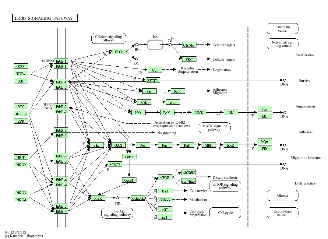
Using known pathway knowledge [1] [2] [3]:

• EGF serves as a source for the pathway and was the experimental treatment.

• EGF is known to initiate signaling, so it can be added and assigned a high score (greater than all other nodes) to emphasize its importance and guide algorithms to start reconstruction from this point. (EGF is currently not in the data). We can assign it a score of 10; chosen empirically.

• EGFR is in the current data. Looking at the pathway, we can see that EGFR directly interacts with EGF in the pathway.

• All other downstream proteins detected in the data can also treated as targets.

• All proteins in the data can be considered active since they correspond to proteins that are active under the given biological condition.

Input node data transformed into a SPRAS-standardized format:

NODE_ID     prize       source  target  active
AAGAB_HUMAN 0.906857382         True   True
... more nodes
EGF_HUMAN   10              True    True    True
EGFR_HUMAN  6.787874699                 True        True
... more nodes

1.8 Finding an Interactome to use

To connect our proteins, we need a background interactome. For this dataset, we merge two protein-protein interaction (PPI) interactomes, prioritizing directed edges when both sources include the same interaction:

• iRefIndex v13 (159,095 undirected interactions)

• PhosphoSitePlus (4,080 directed kinase-substrate interactions)

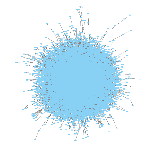
The final network has 15,677 proteins and 157,984 edges (~4k of them are directed), and covers 653 of our 702 prize proteins. The proteins identifiers in the interactome are converted to use UniProt Entry Names.

Interactome data put into a SPRAS-standardized format:

TACC1_HUMAN RUXG_HUMAN      0.736771        U
TACC1_HUMAN KAT2A_HUMAN     0.292198        U
TACC1_HUMAN CKAP5_HUMAN     0.724783        U
TACC1_HUMAN YETS4_HUMAN     0.542597        U
TACC1_HUMAN LSM7_HUMAN      0.714823        U
AURKC_HUMAN TACC1_HUMAN     0.553333        D
TACC1_HUMAN AURKA_HUMAN     0.401165        U
TACC1_HUMAN KDM1A_HUMAN     0.367850        U
TACC1_HUMAN MEMO1_HUMAN     0.367850        U
TACC1_HUMAN HD_HUMAN        0.367850        U
... more edges

Note

Many databases provide interactomes. One example is STRING, which contains known protein-protein interactions across different species. For a broader overview of available interactomes, see Koh et al. (2025). Users can also construct their own interactomes from experimental or curated data.

1.9 This SPRAS-standardized data is already saved into SPRAS

spras/
├── .snakemake/
│   └── log/
│       └── ... snakemake log files ...
├── config/
│   └── ...
├── inputs/
│   ├── phosphosite-irefindex13.0-uniprot.txt # pre-defined in SPRAS already, used by the intermediate.yaml file
│   └── tps-egfr-prizes.txt # pre-defined in SPRAS already, used by the intermediate.yaml file
├── outputs/
│   └── basic/
│       └── ... output files ...

The data used in this part of the tutorial can be found in the supplementary materials under data supplement 2 and supplement 3 [4].

Step 2: Running multiple algorithms

We can begin running multiple pathway reconstruction algorithms.

For this part of the tutorial, we’ll use a pre-defined configuration file that includes additional algorithms and post-analysis steps available in SPRAS. Download it here: Intermediate Config File

Save the file into the config/ folder of your SPRAS installation.

After adding this file, your directory structure will look like this (ignoring the rest of the folders):

spras/
├── .snakemake/
│   └── log/
│       └── ... snakemake log files ...
├── config/
│   ├── basic.yaml
│   ├── intermediate.yaml
│   └── ... other configs ...
├── inputs/
│   ├── phosphosite-irefindex13.0-uniprot.txt # pre-defined in SPRAS already, used by the intermediate.yaml file
│   ├── tps-egfr-prizes.txt # pre-defined in SPRAS already, used by the intermediate.yaml file
│   └── ... other input data ...
├── outputs/
│   └── basic/
│       └── ... output files ...

2.1 Algorithms in SPRAS

SPRAS supports a wide range of algorithms, each designed around different biological assumptions and optimization strategies (See Pathway Reconstruction Methods for SPRAS’s list of integrated algorithms.)

Wrapped algorithms

Each pathway reconstruction algorithm within SPRAS has been wrapped for SPRAS, meaning it has been prepared for the SPRAS framework.

For an algorithm-specific wrapper, the wrapper includes a module that will create and format the input files required by the algorithm using the SPRAS-standardized input data.

Each algorithm has an associated Docker image located on DockerHub that contains all necessary software dependencies needed to run it. For an algorithm-specific wrapper, it contains a module that will call each image to launch a container for a specified parameter combination, set of prepared algorithm-specific inputs and an output filename (raw-pathway.txt).

With each of the raw-pathway.txt files, an algorithm-specific wrapper includes a module that will convert the algorithm-specific format into a standardized SPRAS output format.

2.3 Running SPRAS with multiple algorithms

In the intermediate.yaml configuration file, it is set up to have SPRAS run multiple algorithms with multiple parameter settings on a single dataset.

algorithms:
 - name: "pathlinker"
   include: true
   runs:
     run1:
       k: [1, 10, 100, 1000]

 - name: omicsintegrator2
   include: true
   runs:
     run1:
       b: [4, 10]
       g: [0, 3]
       w: [0.25, 6]

 - name: mincostflow
   include: true
   runs:
     run1:
       capacity: [15, 30]
       flow: [80, 15]

 - name: "strwr"
   include: true
   runs:
     run1:
       alpha: 0.85
       threshold: [100, 200]

 - name: "rwr"
   include: true
   runs:
     run1:
       alpha: 0.85
       threshold: [100, 200]

Note

The full suite of algorithms is described in Pathway Reconstruction Methods. This part of the tutorial uses only a subset.

From the root directory, run the command below from the command line:

snakemake --cores 4 --configfile config/intermediate.yaml

What happens when you run this command

SPRAS will run “slower” when using the intermediate.yaml configuration.

Similar automated steps from the previous tutorial runs behind the scenes for intermediate.yaml. However, this configuration now runs multiple algorithms with different parameter combinations, which takes longer to complete. By increasing the number of cores to 4, it allows Snakemake to parallelize the work locally, speeding up execution when possible. (See Using SPRAS for more information on SPRAS’s parallelization.)

1. Snakemake starts the workflow

Snakemake reads the options set in the intermediate.yaml configuration file and determines which datasets, algorithms, and parameter combinations need to run. It also checks if any post-analysis steps were requested.

2. Creating algorithm-specific inputs

For each algorithm marked as include: true in the configuration, SPRAS generates input files tailored to that algorithm.

In this case, every algorithm is enabled, so SPRAS formats the input files required for each algorithm.

3. Organizing results with parameter hashes

Each <dataset>-<algorithm>-params-<hash> combination gets its own folder created in output/intermediate/.

A matching log file in logs/parameters-<algorithm>-params-<hash>.yaml records the exact parameter values used.

4. Running the algorithm

SPRAS pulls each algorithm’s Docker image from DockerHub if it isn’t already downloaded locally

SPRAS executes each algorithm by launching multiple Docker contatiners using the algorithm-specific Docker image (once for each parameter configuration), sending the prepared input files and specific parameter settings needed for execution.

Each algorithm runs independently within its Docker container and generates an output file named raw-pathway.txt, which contains the reconstructed subnetwork in the algorithm-specific format.

SPRAS then saves these files to the corresponding folder.

5. Standardizing the results

SPRAS parses each of the raw output into a standardized SPRAS format (pathway.txt) and SPRAS saves this file in its corresponding folder.

6. Logging the Snakemake run

Snakemake creates a dated log in .snakemake/log/ This log shows what jobs ran and any errors that occurred during the SPRAS run.

What your directory structure should like after this run:

spras/
├── .snakemake/
│   └── log/
│       └── ... snakemake log files ...
├── config/
│   └── basic.yaml
├── inputs/
│   ├── phosphosite-irefindex13.0-uniprot.txt
│   └── tps-egfr-prizes.txt
├── outputs/
│   └── intermediate/
│       ├── dataset-egfr-merged.pickle
│       ├── egfr-mincostflow-params-42UBTQI/
│       │   ├── pathway.txt
│       │   └── raw-pathway.txt
│       ├── egfr-mincostflow-params-B4P4LUU/
│       │   ├── pathway.txt
│       │   └── raw-pathway.txt
│       ├── egfr-mincostflow-params-KTZPGLQ/
│       │   ├── pathway.txt
│       │   └── raw-pathway.txt
│       ├── egfr-mincostflow-params-MY6UCHG/
│       │   ├── pathway.txt
│       │   └── raw-pathway.txt
│       ├── egfr-omicsintegrator2-params-44PJEHW/
│       │   ├── pathway.txt
│       │   └── raw-pathway.txt
│       ├── egfr-omicsintegrator2-params-4NC62EL/
│       │   ├── pathway.txt
│       │   └── raw-pathway.txt
│       ├── egfr-omicsintegrator2-params-4VRLTK5/
│       │   ├── pathway.txt
│       │   └── raw-pathway.txt
│       ├── egfr-omicsintegrator2-params-52OUGT2/
│       │   ├── pathway.txt
│       │   └── raw-pathway.txt
│       ├── egfr-omicsintegrator2-params-KEVHYWP/
│       │   ├── pathway.txt
│       │   └── raw-pathway.txt
│       ├── egfr-omicsintegrator2-params-RUGOWNI/
│       │   ├── pathway.txt
│       │   └── raw-pathway.txt
│       ├── egfr-omicsintegrator2-params-RVH2YKU/
│       │   ├── pathway.txt
│       │   └── raw-pathway.txt
│       ├── egfr-omicsintegrator2-params-WW2ILRO/
│       │   ├── pathway.txt
│       │   └── raw-pathway.txt
│       ├── egfr-pathlinker-params-7S4SLU6/
│       │   ├── pathway.txt
│       │   └── raw-pathway.txt
│       ├── egfr-pathlinker-params-D4TUKMX/
│       │   ├── pathway.txt
│       │   └── raw-pathway.txt
│       ├── egfr-pathlinker-params-TFORORH/
│       │   ├── pathway.txt
│       │   └── raw-pathway.txt
│       ├── egfr-pathlinker-params-VQL7BDZ/
│       │   ├── pathway.txt
│       │   └── raw-pathway.txt
│       ├── egfr-rwr-params-34NN6EK/
│       │   ├── pathway.txt
│       │   └── raw-pathway.txt
│       ├── egfr-rwr-params-GGZCZBU/
│       │   ├── pathway.txt
│       │   └── raw-pathway.txt
│       ├── egfr-strwr-params-34NN6EK/
│       │   ├── pathway.txt
│       │   └── raw-pathway.txt
│       ├── egfr-strwr-params-GGZCZBU/
│       │   ├── pathway.txt
│       │   └── raw-pathway.txt
│       ├── logs/
│       │   ├── datasets-egfr.yaml
│       │   ├── parameters-mincostflow-params-42UBTQI.yaml
│       │   ├── parameters-mincostflow-params-B4P4LUU.yaml
│       │   ├── parameters-mincostflow-params-KTZPGLQ.yaml
│       │   ├── parameters-mincostflow-params-MY6UCHG.yaml
│       │   ├── parameters-omicsintegrator2-params-44PJEHW.yaml
│       │   ├── parameters-omicsintegrator2-params-4NC62EL.yaml
│       │   ├── parameters-omicsintegrator2-params-4VRLTK5.yaml
│       │   ├── parameters-omicsintegrator2-params-52OUGT2.yaml
│       │   ├── parameters-omicsintegrator2-params-KEVHYWP.yaml
│       │   ├── parameters-omicsintegrator2-params-RUGOWNI.yaml
│       │   ├── parameters-omicsintegrator2-params-RVH2YKU.yaml
│       │   ├── parameters-omicsintegrator2-params-WW2ILRO.yaml
│       │   ├── parameters-pathlinker-params-7S4SLU6.yaml
│       │   ├── parameters-pathlinker-params-D4TUKMX.yaml
│       │   ├── parameters-pathlinker-params-TFORORH.yaml
│       │   ├── parameters-pathlinker-params-VQL7BDZ.yaml
│       │   ├── parameters-rwr-params-34NN6EK.yaml
│       │   ├── parameters-rwr-params-GGZCZBU.yaml
│       │   ├── parameters-strwr-params-34NN6EK.yaml
│       │   └── parameters-strwr-params-GGZCZBU.yaml
│       └── prepared/
│           ├── egfr-mincostflow-inputs/
│           │   ├── edges.txt
│           │   ├── sources.txt
│           │   └── targets.txt
│           ├── egfr-omicsintegrator2-inputs/
│           │   ├── edges.txt
│           │   └── prizes.txt
│           ├── egfr-pathlinker-inputs/
│           │   ├── network.txt
│           │   └── nodetypes.txt
│           ├── egfr-rwr-inputs/
│           │   ├── network.txt
│           │   └── nodes.txt
│           └── egfr-strwr-inputs/
│               ├── network.txt
│               ├── sources.txt
│               └── targets.txt

2.4 Reviewing the pathway.txt files

After running the intermediate configuration file, the output/intermediate/ directory will contain many more subfolders and files.

Again, each pathway.txt file contains the standardized reconstructed subnetworks and can be used at face value, or for further post analysis.

1. Locate the files

Navigate to the output directory output/intermediate/. Inside, you will find subfolders corresponding to each <dataset>-<algorithm>-params-<hash> combination.

2. Open a pathway.txt file

Each file lists the network edges that were reconstructed for that specific run. The format includes columns for the two interacting nodes, the rank, and the edge direction.

For example, the file egfr-mincostflow-params-42UBTQI/pathway.txt contains the following reconstructed subnetwork:

Node1       Node2    Rank     Direction
CBL_HUMAN   EGFR_HUMAN      1       U
EGFR_HUMAN  EGF_HUMAN       1       U
EMD_HUMAN   LMNA_HUMAN      1       U
FYN_HUMAN   KS6A3_HUMAN     1       U
EGF_HUMAN   HDAC6_HUMAN     1       U
HDAC6_HUMAN HS90A_HUMAN     1       U
KS6A3_HUMAN SRC_HUMAN       1       U
EGF_HUMAN   LMNA_HUMAN      1       U
MYH9_HUMAN  S10A4_HUMAN     1       U
EGF_HUMAN   S10A4_HUMAN     1       U
EMD_HUMAN   SRC_HUMAN       1       U

And the file egfr-omicsintegrator1-params-YYFFQV4/pathway.txt contains the following reconstructed subnetwork:

Node1        Node2      Rank    Direction
CBLB_HUMAN   EGFR_HUMAN      1       U
CBL_HUMAN    CD2AP_HUMAN     1       U
CBL_HUMAN    CRKL_HUMAN      1       U
CBL_HUMAN    EGFR_HUMAN      1       U
CBL_HUMAN    PLCG1_HUMAN     1       U
CDK1_HUMAN   NPM_HUMAN       1       D
CHD4_HUMAN   HDAC1_HUMAN     1       U
CHIP_HUMAN   HS90A_HUMAN     1       U
CHIP_HUMAN   P53_HUMAN       1       U
DNMT1_HUMAN  HDAC1_HUMAN     1       U
EGFR_HUMAN   EGF_HUMAN       1       U
EGFR_HUMAN   GRB2_HUMAN      1       U
EIF3B_HUMAN  EIF3G_HUMAN     1       U
FAK1_HUMAN   PAXI_HUMAN      1       U
GAB1_HUMAN   PTN11_HUMAN     1       U
GRB2_HUMAN   KHDR1_HUMAN     1       U
GRB2_HUMAN   PTN11_HUMAN     1       U
GRB2_HUMAN   SHC1_HUMAN      1       U
HDAC1_HUMAN  HDAC2_HUMAN     1       U
HDAC1_HUMAN  P53_HUMAN       1       U
HDAC1_HUMAN  RB_HUMAN        1       U
HDAC1_HUMAN  SIN3A_HUMAN     1       U
HGS_HUMAN    STAM2_HUMAN     1       U
HS90A_HUMAN  STIP1_HUMAN     1       U
HS90A_HUMAN  TEBP_HUMAN      1       U
KHDR1_HUMAN  LCK_HUMAN       1       U
KS6A1_HUMAN  MK01_HUMAN      1       U
MK01_HUMAN   ABI1_HUMAN      1       D
MK01_HUMAN   ERF_HUMAN       1       D
MRE11_HUMAN  RAD50_HUMAN     1       U
P53_HUMAN    TP53B_HUMAN     1       U

Step 3: Use ML post-analysis

Rather than inspecting each output on its own, users may want to understand how the outputs from multiple algorithms and parameter combinations relate to one another when run on the same dataset. SPRAS includes machine learning (ML) post-analysis methods for this: hierarchical agglomerative clustering, principal component analysis, Jaccard similarity, and ensembling.

Note

Each ML method operates on a dataset-specific binary edge-by-subnetwork matrix. Rows represent edges in the union of all reconstructed pathways, and columns represent output subnetworks. An entry indicates whether a given edge appears in a given subnetwork (1 if present, 0 if absent).

3.1 Adding ML post-analysis to the intermediate configuration

To enable the ML analysis, update the analysis section in your configuration file by setting ML to true. Your analysis section in the configuration file should look like this:

analysis:
    ml:
        include: true
        ... (other parameters preset)

ml will perform unsupervised analyses such as principal component analysis, hierarchical agglomerative clustering, ensembling, and jaccard similarity comparisons of the pathways.

Note

The ml section includes configurable parameters that adjust the behavior of these analyses. For the available options, see config.yaml in the config/ folder.

With these updates, SPRAS will run the full ML analyses across all outputs for a given dataset.

After saving the changes in the configuration file, rerun with:

snakemake --cores 4 --configfile config/intermediate.yaml

What happens when you run this command

1. Reusing cached results

Snakemake reads the options set in intermediate.yaml and checks for any requested post-analysis steps. It reuses cached results; here the pathway.txt files generated from the previously executed algorithms on the egfr dataset are reused.

2. Running the ML analysis

SPRAS aggregates all the reconstructed subnetworks produced across the specified algorithms for a given dataset. SPRAS then performs machine learning analyses on each these groups and saves the results in a <dataset>-ml/ (egfr-ml/ in this case) folder.

What your directory structure should like after this run:

spras/
├── .snakemake/
│   └── log/
│       └── ... snakemake log files ...
├── config/
│   └── basic.yaml
├── inputs/
│   ├── phosphosite-irefindex13.0-uniprot.txt
│   └── tps-egfr-prizes.txt
├── outputs/
│   └── intermediate/
│       ├── dataset-egfr-merged.pickle
│       ├── egfr-mincostflow-params-42UBTQI/
│       │   ├── pathway.txt
│       │   └── raw-pathway.txt
│       ├── egfr-mincostflow-params-B4P4LUU/
│       │   ├── pathway.txt
│       │   └── raw-pathway.txt
│       ├── egfr-mincostflow-params-KTZPGLQ/
│       │   ├── pathway.txt
│       │   └── raw-pathway.txt
│       ├── egfr-mincostflow-params-MY6UCHG/
│       │   ├── pathway.txt
│       │   └── raw-pathway.txt
│       ├── egfr-ml/
│       │   ├── ensemble-pathway.txt
│       │   ├── hac-clusters-horizontal.txt
│       │   ├── hac-clusters-vertical.txt
│       │   ├── hac-horizontal.png
│       │   ├── hac-vertical.png
│       │   ├── jaccard-heatmap.png
│       │   ├── jaccard-matrix.txt
│       │   ├── pca-coordinates.txt
│       │   ├── pca-variance.txt
│       │   └── pca.png
│       ├── egfr-omicsintegrator2-params-44PJEHW/
│       │   ├── pathway.txt
│       │   └── raw-pathway.txt
│       ├── egfr-omicsintegrator2-params-4NC62EL/
│       │   ├── pathway.txt
│       │   └── raw-pathway.txt
│       ├── egfr-omicsintegrator2-params-4VRLTK5/
│       │   ├── pathway.txt
│       │   └── raw-pathway.txt
│       ├── egfr-omicsintegrator2-params-52OUGT2/
│       │   ├── pathway.txt
│       │   └── raw-pathway.txt
│       ├── egfr-omicsintegrator2-params-KEVHYWP/
│       │   ├── pathway.txt
│       │   └── raw-pathway.txt
│       ├── egfr-omicsintegrator2-params-RUGOWNI/
│       │   ├── pathway.txt
│       │   └── raw-pathway.txt
│       ├── egfr-omicsintegrator2-params-RVH2YKU/
│       │   ├── pathway.txt
│       │   └── raw-pathway.txt
│       ├── egfr-omicsintegrator2-params-WW2ILRO/
│       │   ├── pathway.txt
│       │   └── raw-pathway.txt
│       ├── egfr-pathlinker-params-7S4SLU6/
│       │   ├── pathway.txt
│       │   └── raw-pathway.txt
│       ├── egfr-pathlinker-params-D4TUKMX/
│       │   ├── pathway.txt
│       │   └── raw-pathway.txt
│       ├── egfr-pathlinker-params-TFORORH/
│       │   ├── pathway.txt
│       │   └── raw-pathway.txt
│       ├── egfr-pathlinker-params-VQL7BDZ/
│       │   ├── pathway.txt
│       │   └── raw-pathway.txt
│       ├── egfr-rwr-params-34NN6EK/
│       │   ├── pathway.txt
│       │   └── raw-pathway.txt
│       ├── egfr-rwr-params-GGZCZBU/
│       │   ├── pathway.txt
│       │   └── raw-pathway.txt
│       ├── egfr-strwr-params-34NN6EK/
│       │   ├── pathway.txt
│       │   └── raw-pathway.txt
│       ├── egfr-strwr-params-GGZCZBU/
│       │   ├── pathway.txt
│       │   └── raw-pathway.txt
│       ├── logs/
│       │   ├── datasets-egfr.yaml
│       │   ├── parameters-mincostflow-params-42UBTQI.yaml
│       │   ├── parameters-mincostflow-params-B4P4LUU.yaml
│       │   ├── parameters-mincostflow-params-KTZPGLQ.yaml
│       │   ├── parameters-mincostflow-params-MY6UCHG.yaml
│       │   ├── parameters-omicsintegrator2-params-44PJEHW.yaml
│       │   ├── parameters-omicsintegrator2-params-4NC62EL.yaml
│       │   ├── parameters-omicsintegrator2-params-4VRLTK5.yaml
│       │   ├── parameters-omicsintegrator2-params-52OUGT2.yaml
│       │   ├── parameters-omicsintegrator2-params-KEVHYWP.yaml
│       │   ├── parameters-omicsintegrator2-params-RUGOWNI.yaml
│       │   ├── parameters-omicsintegrator2-params-RVH2YKU.yaml
│       │   ├── parameters-omicsintegrator2-params-WW2ILRO.yaml
│       │   ├── parameters-pathlinker-params-7S4SLU6.yaml
│       │   ├── parameters-pathlinker-params-D4TUKMX.yaml
│       │   ├── parameters-pathlinker-params-TFORORH.yaml
│       │   ├── parameters-pathlinker-params-VQL7BDZ.yaml
│       │   ├── parameters-rwr-params-34NN6EK.yaml
│       │   ├── parameters-rwr-params-GGZCZBU.yaml
│       │   ├── parameters-strwr-params-34NN6EK.yaml
│       │   └── parameters-strwr-params-GGZCZBU.yaml
│       └── prepared/
│           ├── egfr-mincostflow-inputs/
│           │   ├── edges.txt
│           │   ├── sources.txt
│           │   └── targets.txt
│           ├── egfr-omicsintegrator2-inputs/
│           │   ├── edges.txt
│           │   └── prizes.txt
│           ├── egfr-pathlinker-inputs/
│           │   ├── network.txt
│           │   └── nodetypes.txt
│           ├── egfr-rwr-inputs/
│           │   ├── network.txt
│           │   └── nodes.txt
│           └── egfr-strwr-inputs/
│               ├── network.txt
│               ├── sources.txt
│               └── targets.txt

Step 3.2: Reviewing the ML outputs

Ensembles

1. Open the ensemble file

In your file explorer, go to output/intermediate/egfr-ml/ensemble-pathway.txt and open it locally.

After running multiple algorithms or parameter settings on the same dataset, SPRAS can ensemble the resulting pathways to identify consistent, high-frequency interactions. SPRAS calculates the edge frequency by calculating the proportion of times each edge appears across the outputs.

Node1        Node2   Frequency       Direction
EGF_HUMAN    EGFR_HUMAN      0.3     D
EGF_HUMAN    S10A4_HUMAN     0.25    D
S10A4_HUMAN  MYH9_HUMAN      0.2     D
K7PPA8_HUMAN MDM2_HUMAN      0.15    D
MDM2_HUMAN   P53_HUMAN       0.15    D
S10A4_HUMAN  K7PPA8_HUMAN    0.15    D
K7PPA8_HUMAN SIR1_HUMAN      0.15    D
MDM2_HUMAN   MDM4_HUMAN      0.15    D
MDM4_HUMAN   P53_HUMAN       0.15    D
CD2A2_HUMAN  CDK4_HUMAN      0.15    D
CDK4_HUMAN   RB_HUMAN        0.15    D
MDM2_HUMAN   CD2A2_HUMAN     0.15    D
EP300_HUMAN  P53_HUMAN       0.35    D
K7PPA8_HUMAN EP300_HUMAN     0.15    D
...

High frequency edges indicate interactions consistently recovered by multiple algorithms. Low frequency edges may reflect noise or algorithm-specific connections. Edges that occur across many outputs are less likely to be algorithm-specific artifacts, so ensembling lets you filter for interactions supported by multiple algorithms or parameter settings.

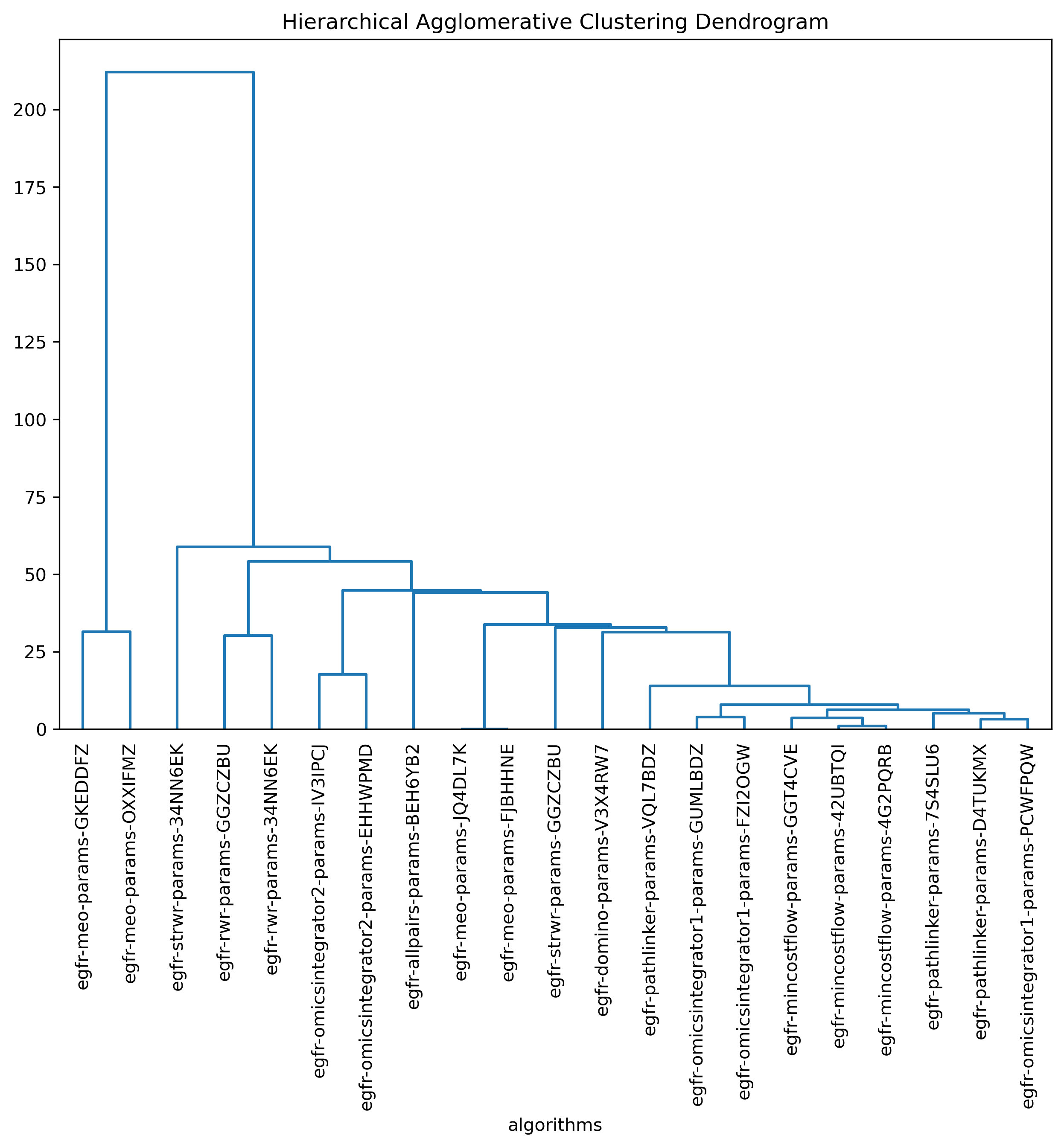
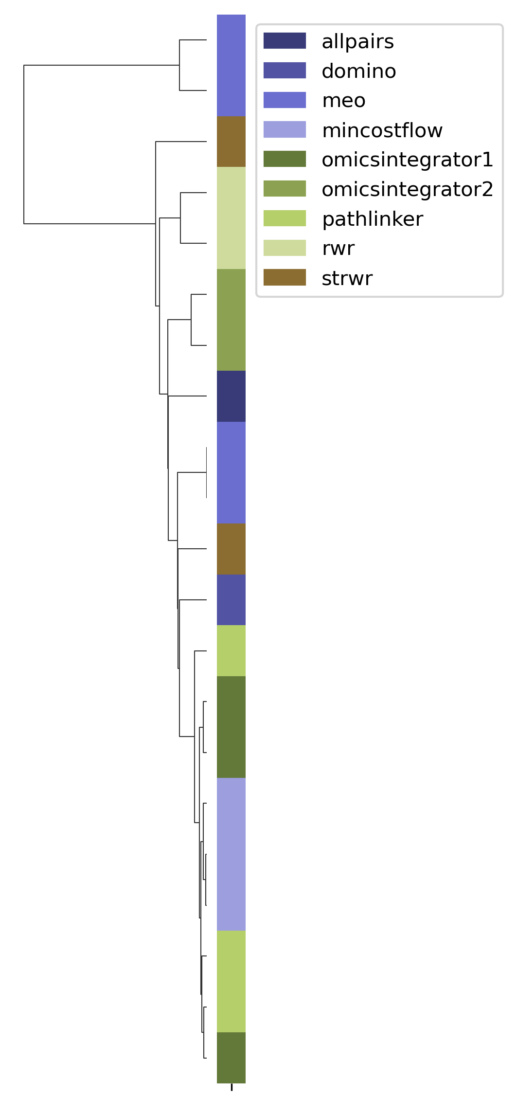
Hierarchical agglomerative clustering

1. Open the hierarchical agglomerative clustering image(s)

In your file explorer, go to output/intermediate/egfr-ml/hac-horizontal.png and/or output/intermediate/egfr-ml/hac-vertical.png and open it locally.

SPRAS includes hierarchical agglomerative clustering to group similar pathways outputs based on shared edges. This helps identify clusters of algorithms that produce comparable subnetworks and highlights distinct reconstruction behaviors.

In the plots below, each branch represents a cluster of related pathways, and shorter distances between branches indicate greater similarity. Tight clusters group algorithms and parameter settings that produce comparable pathway structures, while isolated branches flag outputs that differ from the rest.

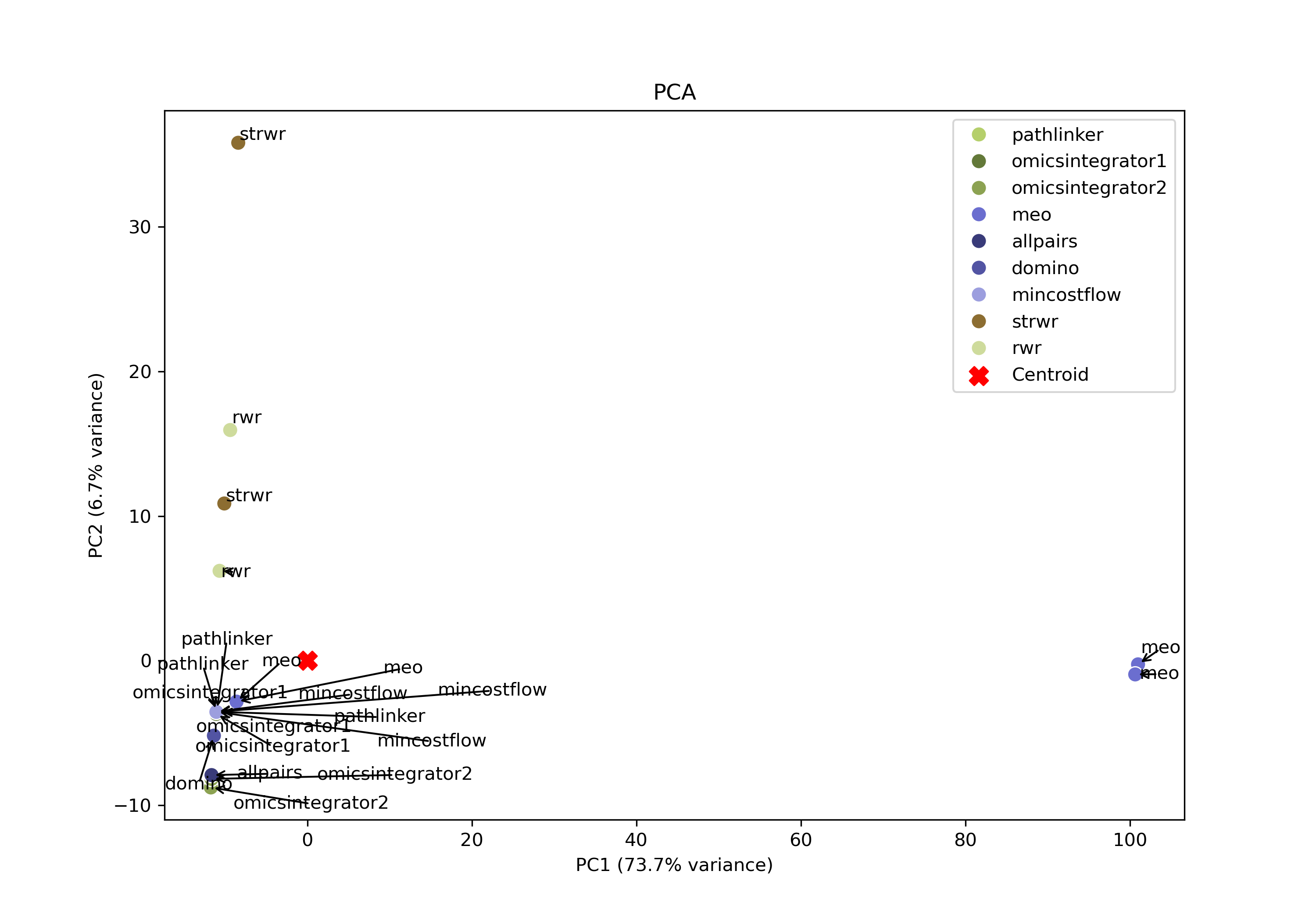
Principal component analysis

1. Open the PCA image

In your file explorer, go to output/intermediate/egfr-ml/pca.png and open it locally.

SPRAS also includes principal component analysis (PCA) to visualize variation across pathway outputs. Each point represents a pathway, placed based on its overall network structure. Pathways that cluster together in PCA space are more similar, while those farther apart differ in their reconstructed subnetworks. PCA may help identify patterns such as clusters of similar algorithms outputs, parameter sensitivities, and/or outlier outputs in a lower lower-dimensional space.

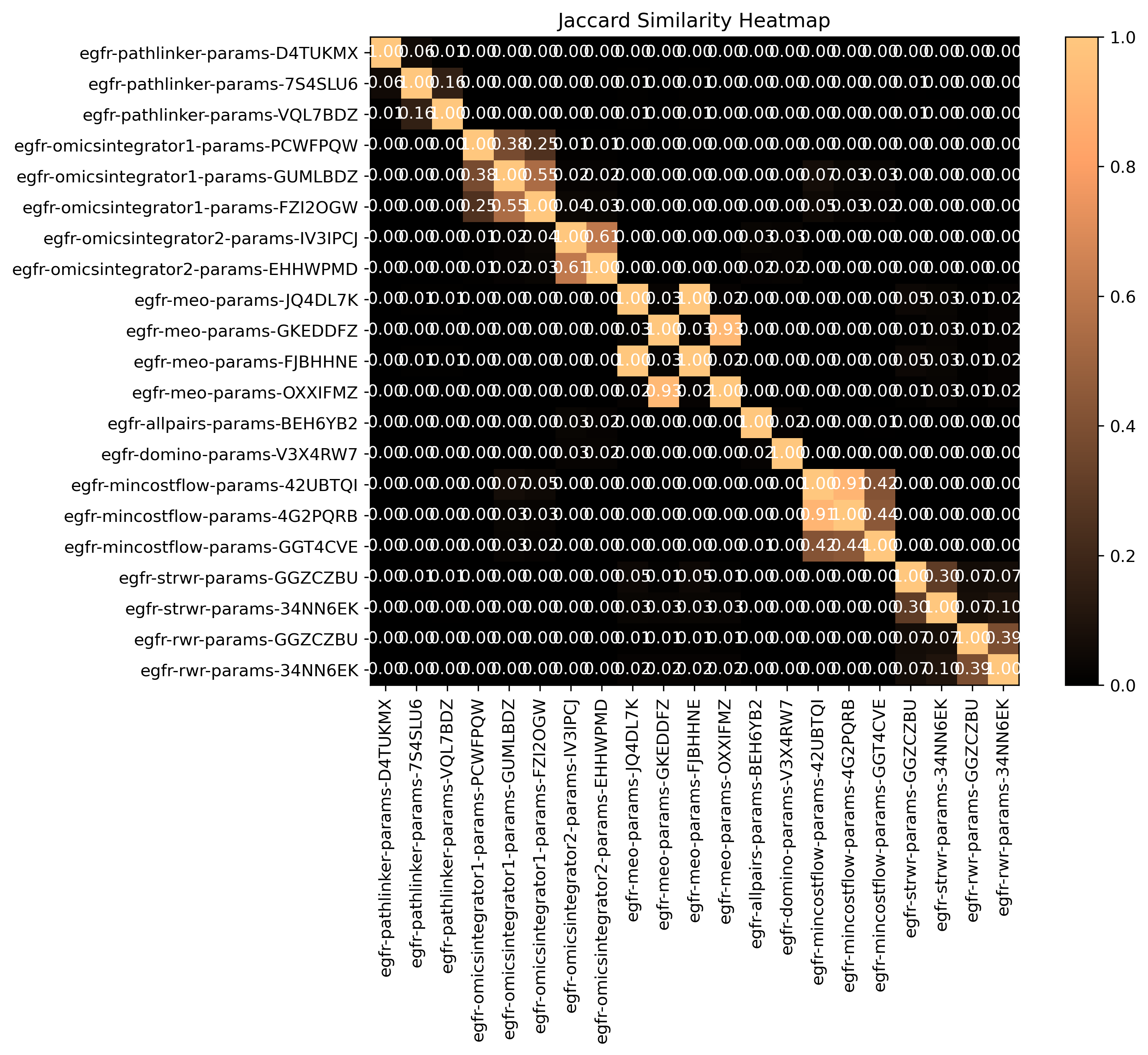
Jaccard similarity

1. Open the jaccard heatmap image

In your file explorer, go to output/intermediate/egfr-ml/jaccard-heatmap.png and open it locally.

SPRAS computes pairwise jaccard similarity between pathway outputs to measure how much overlap exists between their reconstructed subnetworks. The heatmap visualizes how similar the output pathways are between algorithms and their parameter settings. Higher similarity values indicate that pathways share many of the same edges, while lower values suggest distinct reconstructions.

Step 4: Use Evaluation post-analysis

In some cases, users may have a gold standard file that allows them to evaluate the quality of the reconstructed subnetworks generated by pathway reconstruction algorithms.

However, gold standards may not exist for certain types of experimental data where validated ground truth interactions or molecules are unavailable or incomplete. For example, in emerging research areas or poorly characterized biological systems, interactions may not yet be experimentally verified or fully known, making it difficult to define a reliable reference network for evaluation.

Note

A gold standard captures interactions that are already known, but pathway reconstruction is also a tool for discovery. An algorithm that scores well against a gold standard may do so by recovering established interactions while missing novel ones.

4.1 Adding evaluation post-analysis to the intermediate configuration

To enable evaluation, update the analysis section of your configuration file. In the evaluation section, set include and aggregate_per_algorithm to true. Also, in the ml section, set kde, r`emove_empty_pathways, and aggregate_per_algorithm to true. Your analysis section in the configuration file should look like this:

analysis:
   summary:
      include: true
   ml:
      include: true
      aggregate_per_algorithm: true
      kde: true
      remove_empty_pathways: true

   evaluation:
      include: true
      aggregate_per_algorithm: true

Setting aggregate_per_algorithm to true will additionally group post-analysis and evaluations by algorithm per dataset. Without this, outputs from all algorithm per dataset are aggregated together for post-analysis rather than broken out per algorithm.

Within ml, remove_empty_pathways excludes pathways with no nodes or edges from the PCA post analysis. The kde creates a kernel density estimate over the PCA plots.

summary is enabled because evaluation uses summary statistics to break ties between pathways for some of the parameter selection methods (more details further into the tutorial).

We need to delete the existing egfr-ml/ folder before rerunning SPRAS so that Snakemake regenerates the ML outputs with the new customized ML settings. Run this command from the root directory:

rm -rf output/intermediate/egfr-ml/

Note

Snakemake skips steps whose output files already exist, so changes to ML configuration parameters will not trigger a rerun unless the existing ML outputs are removed first.

Automatic re-execution on config changes is a known limitation and is being addressed in ongoing SPRAS development.

The intermediate configuration also includes a gold standard for the EGFR dataset, which is already set up in SPRAS and does not require any setup:

gold_standards:
-
   label: gs_egfr
   node_files: ["gs-egfr.txt"]
   data_dir: "input"
   dataset_labels: ["egfr"]

Note

The gold standard for this dataset consists of nodes only, following the original study. The gold standard nodes are drawn from eight EGFR-related reference pathways [4].

A limitation of this gold standard is its incomplete coverage of EGF signaling pathways. Across the eight reference pathways, typically 5% or fewer of the input nodes appear in any single pathway, and 85% are absent from all eight. This reflects the general incompleteness of curated pathway databases relative to measured signaling responses, rather than a flaw specific to this dataset [4].

With these updates, SPRAS will run the evaluations across all outputs for a given dataset.

After saving the changes in the configuration file, rerun with:

snakemake --cores 4 --configfile config/intermediate.yaml

What happens when you run this command

1. Reusing cached results

Snakemake reads the options set in intermediate.yaml and checks for any requested post-analysis steps. It reuses cached results; here the pathway.txt files generated from the previously executed algorithms on the egfr dataset are reused.

2. Running the ML analysis

SPRAS aggregates all the reconstructed subnetworks produced across the specified algorithms for a given dataset. SPRAS then performs machine learning analyses on each these groups and saves the results in the <dataset>-ml/ (egfr-ml/) folder. It is also going to be running the ML per algorithm for a given dataset. This groups the ML post analysis by algorithm per dataset and produces algorithm specific ML outputs.

3. Running the summary analysis

SPRAS aggregates the pathway.txt files from all selected parameter combinations into a single summary table, saved as egfr-pathway-summary.txt. This is used if any tiebreakers occur during PCA-based parameter selection.

4. Running the evaluation

For each dataset listed in a gold standard’s dataset_labels, SPRAS compares the reconstructed subnetworks against that gold standard using the parameter selection methods enabled in the configuration.

The evaluation runs at two levels: once across all algorithms combined, and once per algorithm. The per-algorithm evaluation depends on per-algorithm ML outputs, which is why aggregate_per_algorithm was set to true in the ml section above. This produces both all-algorithm evaluation files and algorithm-specific evaluation files for each dataset-goldstandard pair.

What your directory structure should like after this run:

spras/
├── .snakemake/
│   └── log/
│       └── ... snakemake log files ...
├── config/
│   └── basic.yaml
├── inputs/
│   ├── phosphosite-irefindex13.0-uniprot.txt
│   └── tps-egfr-prizes.txt
├── outputs/
│   └── intermediate/
│       ├── dataset-egfr-merged.pickle
│       ├── egfr-gs_egfr-eval/
│       │   ├── pr-curve-ensemble-nodes-per-algorithm-nodes.png
│       │   ├── pr-curve-ensemble-nodes-per-algorithm-nodes.txt
│       │   ├── pr-curve-ensemble-nodes.png
│       │   ├── pr-curve-ensemble-nodes.txt
│       │   ├── pr-pca-chosen-pathway-nodes.png
│       │   ├── pr-pca-chosen-pathway-nodes.txt
│       │   ├── pr-pca-chosen-pathway-per-algorithm-nodes.png
│       │   ├── pr-pca-chosen-pathway-per-algorithm-nodes.txt
│       │   ├── pr-per-pathway-for-mincostflow-nodes.png
│       │   ├── pr-per-pathway-for-mincostflow-nodes.txt
│       │   ├── pr-per-pathway-for-omicsintegrator2-nodes.png
│       │   ├── pr-per-pathway-for-omicsintegrator2-nodes.txt
│       │   ├── pr-per-pathway-for-pathlinker-nodes.png
│       │   ├── pr-per-pathway-for-pathlinker-nodes.txt
│       │   ├── pr-per-pathway-for-rwr-nodes.png
│       │   ├── pr-per-pathway-for-rwr-nodes.txt
│       │   ├── pr-per-pathway-for-strwr-nodes.png
│       │   ├── pr-per-pathway-for-strwr-nodes.txt
│       │   ├── pr-per-pathway-nodes.png
│       │   └── pr-per-pathway-nodes.txt
│       ├── egfr-mincostflow-params-42UBTQI/
│       │   ├── pathway.txt
│       │   └── raw-pathway.txt
│       ├── egfr-mincostflow-params-B4P4LUU/
│       │   ├── pathway.txt
│       │   └── raw-pathway.txt
│       ├── egfr-mincostflow-params-KTZPGLQ/
│       │   ├── pathway.txt
│       │   └── raw-pathway.txt
│       ├── egfr-mincostflow-params-MY6UCHG/
│       │   ├── pathway.txt
│       │   └── raw-pathway.txt
│       ├── egfr-ml/
│       │   ├── ensemble-pathway.txt
│       │   ├── hac-clusters-horizontal.txt
│       │   ├── hac-clusters-vertical.txt
│       │   ├── hac-horizontal.png
│       │   ├── hac-vertical.png
│       │   ├── jaccard-heatmap.png
│       │   ├── jaccard-matrix.txt
│       │   ├── mincostflow-ensemble-pathway.txt
│       │   ├── mincostflow-hac-clusters-horizontal.txt
│       │   ├── mincostflow-hac-clusters-vertical.txt
│       │   ├── mincostflow-hac-horizontal.png
│       │   ├── mincostflow-hac-vertical.png
│       │   ├── mincostflow-jaccard-heatmap.png
│       │   ├── mincostflow-jaccard-matrix.txt
│       │   ├── mincostflow-pca-coordinates.txt
│       │   ├── mincostflow-pca-variance.txt
│       │   ├── mincostflow-pca.png
│       │   ├── omicsintegrator2-ensemble-pathway.txt
│       │   ├── omicsintegrator2-hac-clusters-horizontal.txt
│       │   ├── omicsintegrator2-hac-clusters-vertical.txt
│       │   ├── omicsintegrator2-hac-horizontal.png
│       │   ├── omicsintegrator2-hac-vertical.png
│       │   ├── omicsintegrator2-jaccard-heatmap.png
│       │   ├── omicsintegrator2-jaccard-matrix.txt
│       │   ├── omicsintegrator2-pca-coordinates.txt
│       │   ├── omicsintegrator2-pca-variance.txt
│       │   ├── omicsintegrator2-pca.png
│       │   ├── pathlinker-ensemble-pathway.txt
│       │   ├── pathlinker-hac-clusters-horizontal.txt
│       │   ├── pathlinker-hac-clusters-vertical.txt
│       │   ├── pathlinker-hac-horizontal.png
│       │   ├── pathlinker-hac-vertical.png
│       │   ├── pathlinker-jaccard-heatmap.png
│       │   ├── pathlinker-jaccard-matrix.txt
│       │   ├── pathlinker-pca-coordinates.txt
│       │   ├── pathlinker-pca-variance.txt
│       │   ├── pathlinker-pca.png
│       │   ├── pca-coordinates.txt
│       │   ├── pca-variance.txt
│       │   ├── pca.png
│       │   ├── rwr-ensemble-pathway.txt
│       │   ├── rwr-hac-clusters-horizontal.txt
│       │   ├── rwr-hac-clusters-vertical.txt
│       │   ├── rwr-hac-horizontal.png
│       │   ├── rwr-hac-vertical.png
│       │   ├── rwr-jaccard-heatmap.png
│       │   ├── rwr-jaccard-matrix.txt
│       │   ├── rwr-pca-coordinates.txt
│       │   ├── rwr-pca-variance.txt
│       │   ├── rwr-pca.png
│       │   ├── strwr-ensemble-pathway.txt
│       │   ├── strwr-hac-clusters-horizontal.txt
│       │   ├── strwr-hac-clusters-vertical.txt
│       │   ├── strwr-hac-horizontal.png
│       │   ├── strwr-hac-vertical.png
│       │   ├── strwr-jaccard-heatmap.png
│       │   ├── strwr-jaccard-matrix.txt
│       │   ├── strwr-pca-coordinates.txt
│       │   ├── strwr-pca-variance.txt
│       │   └── strwr-pca.png
│       ├── egfr-omicsintegrator2-params-44PJEHW/
│       │   ├── pathway.txt
│       │   └── raw-pathway.txt
│       ├── egfr-omicsintegrator2-params-4NC62EL/
│       │   ├── pathway.txt
│       │   └── raw-pathway.txt
│       ├── egfr-omicsintegrator2-params-4VRLTK5/
│       │   ├── pathway.txt
│       │   └── raw-pathway.txt
│       ├── egfr-omicsintegrator2-params-52OUGT2/
│       │   ├── pathway.txt
│       │   └── raw-pathway.txt
│       ├── egfr-omicsintegrator2-params-KEVHYWP/
│       │   ├── pathway.txt
│       │   └── raw-pathway.txt
│       ├── egfr-omicsintegrator2-params-RUGOWNI/
│       │   ├── pathway.txt
│       │   └── raw-pathway.txt
│       ├── egfr-omicsintegrator2-params-RVH2YKU/
│       │   ├── pathway.txt
│       │   └── raw-pathway.txt
│       ├── egfr-omicsintegrator2-params-WW2ILRO/
│       │   ├── pathway.txt
│       │   └── raw-pathway.txt
│       ├── egfr-pathlinker-params-7S4SLU6/
│       │   ├── pathway.txt
│       │   └── raw-pathway.txt
│       ├── egfr-pathlinker-params-D4TUKMX/
│       │   ├── pathway.txt
│       │   └── raw-pathway.txt
│       ├── egfr-pathlinker-params-TFORORH/
│       │   ├── pathway.txt
│       │   └── raw-pathway.txt
│       ├── egfr-pathlinker-params-VQL7BDZ/
│       │   ├── pathway.txt
│       │   └── raw-pathway.txt
│       ├── egfr-pathway-summary.txt
│       ├── egfr-rwr-params-34NN6EK/
│       │   ├── pathway.txt
│       │   └── raw-pathway.txt
│       ├── egfr-rwr-params-GGZCZBU/
│       │   ├── pathway.txt
│       │   └── raw-pathway.txt
│       ├── egfr-strwr-params-34NN6EK/
│       │   ├── pathway.txt
│       │   └── raw-pathway.txt
│       ├── egfr-strwr-params-GGZCZBU/
│       │   ├── pathway.txt
│       │   └── raw-pathway.txt
│       ├── gs-gs_egfr-merged.pickle
│       ├── logs/
│       │   ├── datasets-egfr.yaml
│       │   ├── parameters-mincostflow-params-42UBTQI.yaml
│       │   ├── parameters-mincostflow-params-B4P4LUU.yaml
│       │   ├── parameters-mincostflow-params-KTZPGLQ.yaml
│       │   ├── parameters-mincostflow-params-MY6UCHG.yaml
│       │   ├── parameters-omicsintegrator2-params-44PJEHW.yaml
│       │   ├── parameters-omicsintegrator2-params-4NC62EL.yaml
│       │   ├── parameters-omicsintegrator2-params-4VRLTK5.yaml
│       │   ├── parameters-omicsintegrator2-params-52OUGT2.yaml
│       │   ├── parameters-omicsintegrator2-params-KEVHYWP.yaml
│       │   ├── parameters-omicsintegrator2-params-RUGOWNI.yaml
│       │   ├── parameters-omicsintegrator2-params-RVH2YKU.yaml
│       │   ├── parameters-omicsintegrator2-params-WW2ILRO.yaml
│       │   ├── parameters-pathlinker-params-7S4SLU6.yaml
│       │   ├── parameters-pathlinker-params-D4TUKMX.yaml
│       │   ├── parameters-pathlinker-params-TFORORH.yaml
│       │   ├── parameters-pathlinker-params-VQL7BDZ.yaml
│       │   ├── parameters-rwr-params-34NN6EK.yaml
│       │   ├── parameters-rwr-params-GGZCZBU.yaml
│       │   ├── parameters-strwr-params-34NN6EK.yaml
│       │   └── parameters-strwr-params-GGZCZBU.yaml
│       └── prepared/
│           ├── egfr-mincostflow-inputs/
│           │   ├── edges.txt
│           │   ├── sources.txt
│           │   └── targets.txt
│           ├── egfr-omicsintegrator2-inputs/
│           │   ├── edges.txt
│           │   └── prizes.txt
│           ├── egfr-pathlinker-inputs/
│           │   ├── network.txt
│           │   └── nodetypes.txt
│           ├── egfr-rwr-inputs/
│           │   ├── network.txt
│           │   └── nodes.txt
│           └── egfr-strwr-inputs/
│               ├── network.txt
│               ├── sources.txt
│               └── targets.txt

4.2 What is parameter selection?

Parameter selection refers to the process of determining which parameter combinations should be used for evaluation on a gold standard dataset. Each parameter selection method has its own corresponding evaluation procedure.

Note

There is no single principled way to decide which outputs to evaluate, so SPRAS provides several parameter selection strategies instead of committing to one. Some strategies pick a single representative output for each algorithm, while others evaluate across the full set of parameter combinations.

Parameter selection also guards against overtuning. Algorithms differ in how many parameters they expose and how much they can be tuned to get a better answer, so comparing them on a representative output rather than on the full sweep puts them on some fairer footing.

Selecting a representative output also measures how an algorithm typically behaves rather than its best run, which is a better basis for judging an algorithm in practice, where the ideal parameters for a new dataset are not known in advance.

Parameter selection is handled in the evaluation code, which supports multiple parameter selection strategies. A user can enable evaluation (by setting evaluation include: true) and it will run all of the parameter selection code.

Note

Some parameter selection features are still under development and will be added in future SPRAS releases.

PCA-based parameter selection

The PCA-based approach identifies a representative parameter setting for each pathway reconstruction algorithm on a given dataset. It selects the single parameter combination that best captures the central trend of an algorithm’s reconstruction behavior.

For each algorithm, all reconstructed subnetworks are projected into an algorithm-specific 2D PCA space based on the set of edges produced by the respective parameter combinations for that algorithm. This projection summarizes how the algorithm’s outputs vary across different parameter combinations, allowing patterns in the outputs to be visualized in a lower-dimensional space.

Within each PCA space, a kernel density estimate (KDE) is computed over the projected points to identify regions of high density. The output closest to the highest KDE peak is selected as the most representative parameter setting, as it corresponds to the region where the algorithm most consistently produces similar subnetworks.

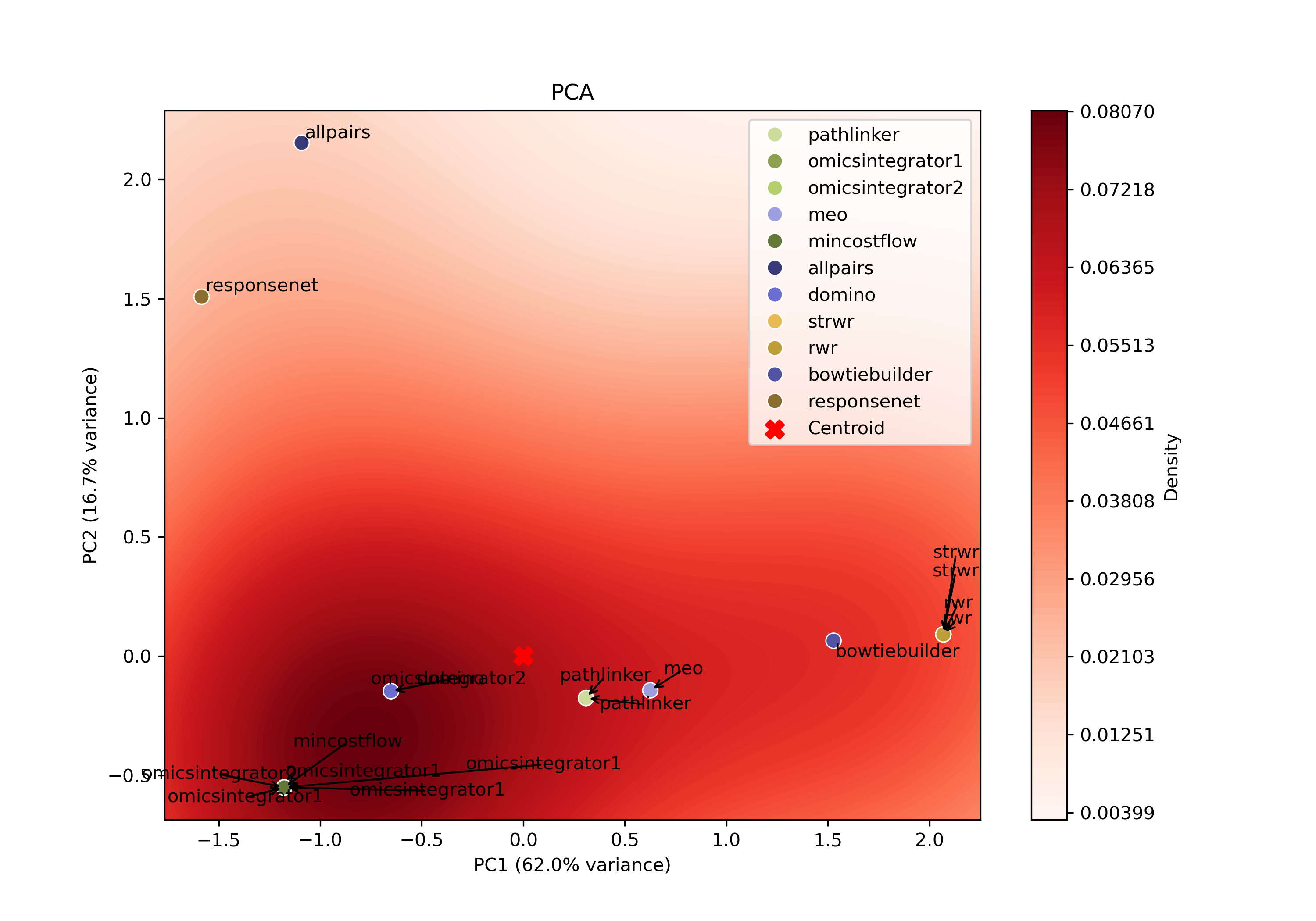
If two or more pathways are equally close to the highest peak of the KDE, SPRAS resolves the tie by:

• Choosing the smallest pathway (fewest nodes and edges).

• If a tie remains, choosing the first pathway alphabetically by name.

The chosen output subnetwork is then compared to the gold standard, and its precision and recall are measured.

Ensemble network-based parameter selection

The ensemble-based approach combines results from all parameter settings for each pathway reconstruction algorithm on a given dataset. Instead of focusing on a single “best” parameter combination, it summarizes the algorithm’s overall reconstruction behavior across parameters.

All reconstructed subnetworks are merged into algorithm-specific ensemble networks, where each edge weight reflects how frequently that interaction appears across the outputs. Edges that occur more often are assigned higher weights, highlighting interactions that are most consistently recovered by the algorithm.

These consensus networks help identify the core patterns and overall stability of an algorithm’s output’s without needing to choose a single parameter setting (no clear optimal parameter combination could exists).

For each algorithm-specific ensemble network, SPRAS generates a precision-recall curve by treating edge frequencies as thresholds and evaluating each ensemble network against the dataset’s associated gold standard.

All Plausible Parameters (No parameter selection)

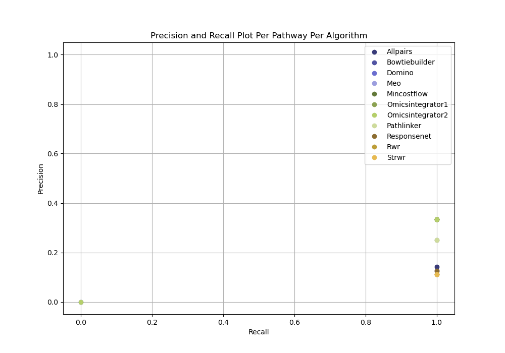
The all plausible parameters approach evaluates all parameter combinations without selecting a representative subset or ensembling. This method provides an holistic view of algorithm performance by evaluating every output. For each algorithm and dataset, we compute precision and recall for every subnetwork. This allows us to measure reconstruction performance across the full range of parameter settings and observe each algorithm’s full range of capabilities.

4.4 Reviewing the evalaution outputs

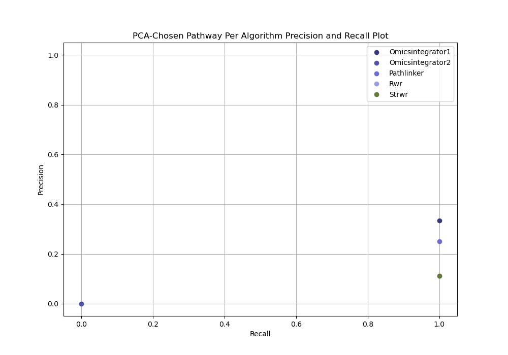
PCA-based parameter selection

1. Open the PCA chosen parameter selection evaluation

In your file explorer, go to output/intermediate/egfr-gs_egfr-eval/pr-per-pathway-nodes.png and open it locally.

PCA-based parameter selection computes a precision and recall for a single reconstructed network selected using PCA from all reconstructed networks for an algorithm for given dataset.

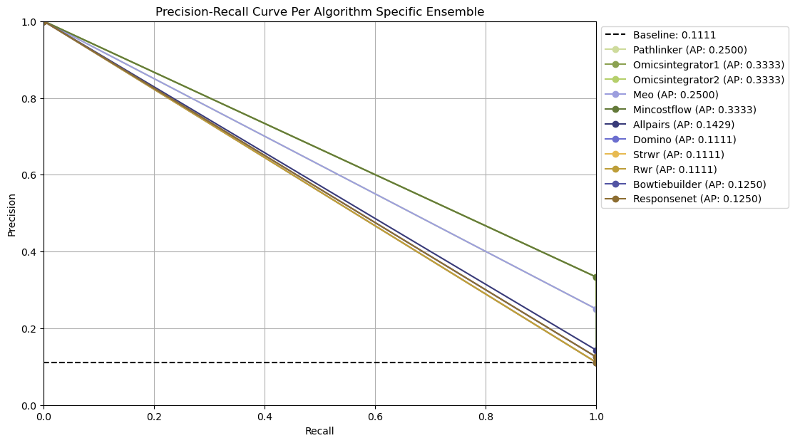
Ensemble network-based parameter selection

1. Open the Ensemble-based parameter selection evalaution

In your file explorer, go to output/intermediate/egfr-gs_egfr-eval/pr-curve-ensemble-nodes-per-algorithm-nodes.png and open it locally.

Ensemble-based parameter selection generates precision-recall curves by thresholding on the frequency of edges across an ensemble of reconstructed networks for an algorithm for given dataset.

All Plausible Parameters (No parameter selection)

1. Open the all plausible parameters (no parameter selection) evalaution

In your file explorer, go to output/intermediate/egfr-gs_egfr-eval/pr-per-pathway-nodes.png and open it locally.

For each pathway, evaluation can be run independently of any parameter selection method to directly inspect precision and recall for each reconstructed network from a given dataset.

References

[1]

Kanehisa, M., Furumichi, M., Sato, Y., Matsuura, Y. and Ishiguro-Watanabe, M.; KEGG: biological systems database as a model of the real world. Nucleic Acids Res. 53, D672-D677 (2025).

[2]

Kanehisa, M; Toward understanding the origin and evolution of cellular organisms. Protein Sci. 28, 1947-1951 (2019)

[3]

Kanehisa, M. and Goto, S.; KEGG: Kyoto Encyclopedia of Genes and Genomes. Nucleic Acids Res. 28, 27-30 (2000).

[4] (1,2,3,4)

Köksal AS, Beck K, Cronin DR, McKenna A, Camp AND, Srivastava S, MacGilvray ME, Bodík R, Wolf-Yadlin A, Fraenkel E, Fisher J, Gitter A. Synthesizing Signaling Pathways from Temporal Phosphoproteomic Data. Cell Rep. 2018 Sep 25;24(13):3607-3618. doi: 10.1016/j.celrep.2018.08.085. PMID: 30257219; PMCID: PMC6295338.